Examples
A number of examples of how to use Nempy are provided below. Examples 1 to 5 are simple and aim introduce various market features that can be modelled with Nempy in an easy to understand way, the dispatch and pricing outcomes are explained in inline comments where the results are printed. Examples 6 and 7 show how to use the historical data input preparation tools provided with Nempy to recreate historical dispatch intervals. Historical dispatch and pricing outcomes can be difficult to interpret as they are usually the result of complex interactions between the many features of the dispatch process, for these example the results are plotted in comparison to historical price outcomes. Example 8 demonstrates how the outputs of one dispatch interval can be used as the initial conditions of the next dispatch interval to create a time sequential model, additionally the current limitations with the approach are briefly discussed.
1. Bid stack equivalent market
This example implements a one region bid stack model of an electricity market. Under the bid stack model, generators are dispatched according to their bid prices, from cheapest to most expensive, until all demand is satisfied. No loss factors, ramping constraints or other factors are considered.
 1import pandas as pd
 2from nempy import markets
 3
 4# Volume of each bid, number of bands must equal number of bands in price_bids.
 5volume_bids = pd.DataFrame({
 6    'unit': ['A', 'B'],
 7    '1': [20.0, 50.0],  # MW
 8    '2': [20.0, 30.0],  # MW
 9    '3': [5.0, 10.0]  # More bid bands could be added.
10})
11
12# Price of each bid, bids must be monotonically increasing.
13price_bids = pd.DataFrame({
14    'unit': ['A', 'B'],
15    '1': [50.0, 50.0],  # $/MW
16    '2': [60.0, 55.0],  # $/MW
17    '3': [100.0, 80.0]  # . . .
18})
19
20# Other unit properties
21unit_info = pd.DataFrame({
22    'unit': ['A', 'B'],
23    'region': ['NSW', 'NSW'],  # MW
24})
25
26# The demand in the region\s being dispatched
27demand = pd.DataFrame({
28    'region': ['NSW'],
29    'demand': [115.0]  # MW
30})
31
32# Create the market model
33market = markets.SpotMarket(unit_info=unit_info, market_regions=['NSW'])
34market.set_unit_volume_bids(volume_bids)
35market.set_unit_price_bids(price_bids)
36market.set_demand_constraints(demand)
37
38# Calculate dispatch and pricing
39market.dispatch()
40
41# Return the total dispatch of each unit in MW.
42print(market.get_unit_dispatch())
43#   unit service  dispatch
44# 0    A  energy      35.0
45# 1    B  energy      80.0
46
47# Understanding the dispatch results: Unit A's first bid is 20 MW at 50 $/MW,
48# and unit B's first bid is 50 MW at 50 $/MW, as demand for electricity is
49# 115 MW both these bids are need to meet demand and so both will be fully
50# dispatched. The next cheapest bid is 30 MW at 55 $/MW from unit B, combining
51# this with the first two bids we get 100 MW of generation, so all of this bid
52# will be dispatched. The next cheapest bid is 20 MW at 60 $/MW from unit A, by
53# dispatching 15 MW of this bid we get a total of 115 MW generation, and supply
54# meets demand so no more bids need to be dispatched. Adding up the dispatched
55# bids from each generator we can see that unit A will be dispatch for 35 MW
56# and unit B will be dispatch for 80 MW, as given by our bid stack market model.
57
58# Return the price of energy in each region.
59print(market.get_energy_prices())
60#   region  price
61# 0    NSW   60.0
62
63# Understanding the pricing result: In this case the marginal bid, the bid
64# that would be dispatch if demand increased is the 60 $/MW bid from unit
65# B, thus this bid sets the price.
66
67# Additional Detail: The above is a simplified interpretation
68# of the pricing result, note that the price is actually taken from the
69# underlying linear problem's shadow price for the supply equals demand constraint.
70# The way the problem is formulated if supply sits exactly between two bids,
71# for example at 120.0 MW, then the price is set by the lower rather
72# than the higher bid. Note, in practical use cases if the demand is a floating point
73# number this situation is unlikely to occur.
2. Unit loss factors, capacities and ramp rates
A simple example with two units in a one region market, units are given loss factors, capacity values and ramp rates. The effects of loss factors on dispatch and market prices are explained.
 1import pandas as pd
 2from nempy import markets
 3
 4# Volume of each bid, number of bands must equal number of bands in price_bids.
 5volume_bids = pd.DataFrame({
 6    'unit': ['A', 'B'],
 7    '1': [20.0, 50.0],  # MW
 8    '2': [25.0, 30.0],  # MW
 9    '3': [5.0, 10.0]  # More bid bands could be added.
10})
11
12# Price of each bid, bids must be monotonically increasing.
13price_bids = pd.DataFrame({
14    'unit': ['A', 'B'],
15    '1': [40.0, 50.0],  # $/MW
16    '2': [60.0, 55.0],  # $/MW
17    '3': [100.0, 80.0]  # . . .
18})
19
20# Factors limiting unit output.
21unit_limits = pd.DataFrame({
22    'unit': ['A', 'B'],
23    'initial_output': [0.0, 0.0],  # MW
24    'capacity': [55.0, 90.0],  # MW
25    'ramp_up_rate': [600.0, 720.0],  # MW/h
26    'ramp_down_rate': [600.0, 720.0]  # MW/h
27})
28
29# Other unit properties including loss factors.
30unit_info = pd.DataFrame({
31    'unit': ['A', 'B'],
32    'region': ['NSW', 'NSW'],  # MW
33    'loss_factor': [0.9, 0.95]
34})
35
36# The demand in the region\s being dispatched.
37demand = pd.DataFrame({
38    'region': ['NSW'],
39    'demand': [100.0]  # MW
40})
41
42# Create the market model
43market = markets.SpotMarket(unit_info=unit_info,
44                            market_regions=['NSW'])
45market.set_unit_volume_bids(volume_bids)
46market.set_unit_price_bids(price_bids)
47market.set_unit_bid_capacity_constraints(
48    unit_limits.loc[:, ['unit', 'capacity']])
49market.set_unit_ramp_rate_constraints(
50    unit_limits.loc[:, ['unit', 'initial_output', 'ramp_up_rate', 'ramp_down_rate']])
51market.set_demand_constraints(demand)
52
53# Calculate dispatch and pricing
54market.dispatch()
55
56# Return the total dispatch of each unit in MW.
57print(market.get_unit_dispatch())
58#   unit service  dispatch
59# 0    A  energy      40.0
60# 1    B  energy      60.0
61
62# Understanding the dispatch results: In this example unit loss factors are
63# provided, that means the cost of a bid in the dispatch optimisation is
64# the bid price divided by the unit loss factor. However, loss factors do
65# not effect the amount of generation a unit can supply, this is because the
66# regional demand already factors in intra regional losses. The cheapest bid is
67# from unit A with 20 MW at 44.44 $/MW (after loss factor), this will be
68# fully dispatched. The next cheapest bid is from unit B with 50 MW at
69# 52.63 $/MW, again fully dispatch. The next cheapest is unit B with 30 MW at
70# 57.89 $/MW, however, unit B starts the interval at a dispatch level of 0.0 MW
71# and can ramp at speed of 720 MW/hr, the default dispatch interval of Nempy
72# is 5 min, so unit B can at most produce 60 MW by the end of the
73# dispatch interval, this means only 10 MW of the second bid from unit B can be
74# dispatched. Finally, the last bid that needs to be dispatch for supply to
75# equal demand is from unit A with 25 MW at 66.67 $/MW, only 20 MW of this
76# bid is needed. Adding together the bids from each unit we can see that
77# unit A is dispatch for a total of 40 MW and unit B for a total of 60 MW.
78
79# Return the price of energy in each region.
80print(market.get_energy_prices())
81#   region  price
82# 0    NSW  66.67
83
84# Understanding the pricing result: In this case the marginal bid, the bid
85# that would be dispatch if demand increased is the second bid from unit A,
86# after adjusting for the loss factor this bid has a price of 66.67 $/MW bid,
87# and this bid sets the price.
3. Interconnector with losses
A simple example demonstrating how to implement a two region market with an interconnector. The interconnector is modelled simply, with a fixed percentage of losses. To make the interconnector flow and loss calculation easy to understand a single unit is modelled in the NSW region, NSW demand is set zero, and VIC region demand is set to 90 MW, thus all the power to meet VIC demand must flow across the interconnetcor.
  1import pandas as pd
  2from nempy import markets
  3
  4# The only generator is located in NSW.
  5unit_info = pd.DataFrame({
  6    'unit': ['A'],
  7    'region': ['NSW']  # MW
  8})
  9
 10# Create a market instance.
 11market = markets.SpotMarket(unit_info=unit_info, market_regions=['NSW', 'VIC'])
 12
 13# Volume of each bids.
 14volume_bids = pd.DataFrame({
 15    'unit': ['A'],
 16    '1': [100.0]  # MW
 17})
 18
 19market.set_unit_volume_bids(volume_bids)
 20
 21# Price of each bid.
 22price_bids = pd.DataFrame({
 23    'unit': ['A'],
 24    '1': [50.0]  # $/MW
 25})
 26
 27market.set_unit_price_bids(price_bids)
 28
 29# NSW has no demand but VIC has 90 MW.
 30demand = pd.DataFrame({
 31    'region': ['NSW', 'VIC'],
 32    'demand': [0.0, 90.0]  # MW
 33})
 34
 35market.set_demand_constraints(demand)
 36
 37# There is one interconnector between NSW and VIC. Its nominal direction is towards VIC.
 38interconnectors = pd.DataFrame({
 39    'interconnector': ['little_link'],
 40    'to_region': ['VIC'],
 41    'from_region': ['NSW'],
 42    'max': [100.0],
 43    'min': [-120.0]
 44})
 45
 46market.set_interconnectors(interconnectors)
 47
 48
 49# The interconnector loss function. In this case losses are always 5 % of line flow.
 50def constant_losses(flow):
 51    return abs(flow) * 0.05
 52
 53
 54# The loss function on a per interconnector basis. Also details how the losses should be proportioned to the
 55# connected regions.
 56loss_functions = pd.DataFrame({
 57    'interconnector': ['little_link'],
 58    'from_region_loss_share': [0.5],  # losses are shared equally.
 59    'loss_function': [constant_losses]
 60})
 61
 62# The points to linearly interpolate the loss function between. In this example the loss function is linear so only
 63# three points are needed, but if a non linear loss function was used then more points would be better.
 64interpolation_break_points = pd.DataFrame({
 65    'interconnector': ['little_link', 'little_link', 'little_link'],
 66    'loss_segment': [1, 2, 3],
 67    'break_point': [-120.0, 0.0, 100]
 68})
 69
 70market.set_interconnector_losses(loss_functions, interpolation_break_points)
 71
 72# Calculate dispatch.
 73market.dispatch()
 74
 75# Return interconnector flow and losses.
 76print(market.get_interconnector_flows())
 77#   interconnector       flow    losses
 78# 0    little_link  92.307692  4.615385
 79
 80# Understanding the interconnector flows: Losses are modelled as extra demand
 81# in the regions on either side of the interconnector, in this case the losses
 82# are split evenly between the regions. All demand in VIC must be supplied
 83# across the interconnector, and losses in VIC will add to the interconnector
 84# flow required, so we can write the equation:
 85#
 86# flow = vic_demand + flow * loss_pct_vic
 87# flow - flow * loss_pct_vic = vic_demand
 88# flow * (1 - loss_pct_vic) = vic_demand
 89# flow = vic_demand / (1 - loss_pct_vic)
 90#
 91# Since interconnector losses are 5% and half occur in VIC the
 92# loss_pct_vic = 2.5%. Thus:
 93#
 94# flow = 90 / (1 - 0.025) = 92.31
 95#
 96# Knowing the interconnector flow we can work out total losses
 97#
 98# losses = flow * loss_pct
 99# losses = 92.31 * 0.05 = 4.62
100
101# Return the total dispatch of each unit in MW.
102print(market.get_unit_dispatch())
103#   unit service   dispatch
104# 0    A  energy  94.615385
105
106# Understanding dispatch results: Unit A must be dispatch to
107# meet supply in VIC plus all interconnector losses, therefore
108# dispatch is 90.0 + 4.62 = 94.62.
109
110# Return the price of energy in each region.
111print(market.get_energy_prices())
112#   region      price
113# 0    NSW  50.000000
114# 1    VIC  52.564103
115
116# Understanding pricing results: The marginal cost of supply in NSW is simply
117# the cost of unit A's bid. However, the marginal cost of supply in VIC also
118# includes the cost of paying for interconnector losses.
4. Dynamic non-linear interconnector losses
This example demonstrates how to model regional demand dependant interconnector loss functions as decribed in the AEMO
Marginal Loss Factors documentation section 3 to 5.
To make the interconnector flow and loss calculation easy to understand a single unit is modelled in the NSW region,
NSW demand is set zero, and VIC region demand is set to 800 MW, thus all the power to meet VIC demand must flow across
the interconnetcor.
  1import pandas as pd
  2from nempy import markets
  3from nempy.historical_inputs import interconnectors as interconnector_inputs
  4
  5
  6# The only generator is located in NSW.
  7unit_info = pd.DataFrame({
  8    'unit': ['A'],
  9    'region': ['NSW']  # MW
 10})
 11
 12# Create a market instance.
 13market = markets.SpotMarket(unit_info=unit_info,
 14                            market_regions=['NSW', 'VIC'])
 15
 16# Volume of each bids.
 17volume_bids = pd.DataFrame({
 18    'unit': ['A'],
 19    '1': [1000.0]  # MW
 20})
 21
 22market.set_unit_volume_bids(volume_bids)
 23
 24# Price of each bid.
 25price_bids = pd.DataFrame({
 26    'unit': ['A'],
 27    '1': [50.0]  # $/MW
 28})
 29
 30market.set_unit_price_bids(price_bids)
 31
 32# NSW has no demand but VIC has 800 MW.
 33demand = pd.DataFrame({
 34    'region': ['NSW', 'VIC'],
 35    'demand': [0.0, 800.0],  # MW
 36    'loss_function_demand': [0.0, 800.0]  # MW
 37})
 38
 39market.set_demand_constraints(demand.loc[:, ['region', 'demand']])
 40
 41# There is one interconnector between NSW and VIC.
 42# Its nominal direction is towards VIC.
 43interconnectors = pd.DataFrame({
 44    'interconnector': ['VIC1-NSW1'],
 45    'to_region': ['VIC'],
 46    'from_region': ['NSW'],
 47    'max': [1000.0],
 48    'min': [-1200.0]
 49})
 50
 51market.set_interconnectors(interconnectors)
 52
 53# Create a demand dependent loss function.
 54# Specify the demand dependency
 55demand_coefficients = pd.DataFrame({
 56    'interconnector': ['VIC1-NSW1', 'VIC1-NSW1'],
 57    'region': ['NSW1', 'VIC1'],
 58    'demand_coefficient': [0.000021734, -0.000031523]})
 59
 60# Specify the loss function constant and flow coefficient.
 61interconnector_coefficients = pd.DataFrame({
 62    'interconnector': ['VIC1-NSW1'],
 63    'loss_constant': [1.0657],
 64    'flow_coefficient': [0.00017027],
 65    'from_region_loss_share': [0.5]})
 66
 67# Create loss functions on per interconnector basis.
 68loss_functions = interconnector_inputs.create_loss_functions(
 69    interconnector_coefficients, demand_coefficients,
 70    demand.loc[:, ['region', 'loss_function_demand']])
 71
 72# The points to linearly interpolate the loss function between.
 73interpolation_break_points = pd.DataFrame({
 74    'interconnector': 'VIC1-NSW1',
 75    'loss_segment': [1, 2, 3, 4, 5, 6, 7, 8, 9, 10, 11, 12],
 76    'break_point': [-1200.0, -1000.0, -800.0, -600.0, -400.0, -200.0,
 77                    0.0, 200.0, 400.0, 600.0, 800.0, 1000]
 78})
 79
 80market.set_interconnector_losses(loss_functions,
 81                                 interpolation_break_points)
 82
 83# Calculate dispatch.
 84market.dispatch()
 85
 86# Return interconnector flow and losses.
 87print(market.get_interconnector_flows())
 88#   interconnector        flow      losses
 89# 0      VIC1-NSW1  860.102737  120.205473
 90
 91# Understanding the interconnector flows: In this case it is not simple to
 92# analytically derive and explain the interconnector flow result. The loss
 93# model is constructed within the underlying mixed integer linear problem
 94# as set of constraints and the interconnector flow and losses are
 95# determined as part of the problem solution. However, the loss model can
 96# be explained at a high level, and the results shown to be consistent. The
 97# first step in the interconnector model is to drive the loss function as a
 98# function  of regional demand, which is a pre-market model creation step, the
 99# mathematics is explained in
100# docs/pdfs/Marginal Loss Factors for the 2020-21 Financial year.pdf. The loss
101# function is then evaluated at the given break points and linearly interpolated
102# between those points in the market model. So for our model the losses are
103# interpolated between 800 MW and 1000 MW. We can show the losses are consistent
104# with this approach:
105#
106# Losses at a flow of 800 MW
107print(loss_functions['loss_function'].iloc[0](800))
108# 107.0464
109# Losses at a flow of 1000 MW
110print(loss_functions['loss_function'].iloc[0](1000))
111# 150.835
112# Then interpolating by taking the weighted sum of the two losses based on the
113# relative difference between the actual flow and the interpolation break points:
114# Weighting of 800 MW break point = 1 - ((860.102737 - 800.0)/(1000 - 800))
115# Weighting of 800 MW break point = 0.7
116# Weighting of 1000 MW break point = 1 - ((1000 - 860.102737)/(1000 - 800))
117# Weighting of 1000 MW break point = 0.3
118# Weighed sum of losses = 107.0464 * 0.7 + 150.835 * 0.3 = 120.18298
119#
120# We can also see that the flow and loss results are consistent with the supply
121# equals demand constraint, all demand in the VIC region is supplied by the
122# interconnector, so the interconnector flow minus the VIC region interconnector
123# losses should equal the VIC region demand. Note that the VIC region loss
124# share is 50%:
125# VIC region demand = interconnector flow - losses * VIC region loss share
126# 800 = 860.102737 - 120.205473 * 0.5
127# 800 = 800
128
129# Return the total dispatch of each unit in MW.
130print(market.get_unit_dispatch())
131#   unit service    dispatch
132# 0    A  energy  920.205473
133
134# Understanding the dispatch results: Unit A is the only generator and it must
135# be dispatched to meet demand plus losses:
136# dispatch = VIC region demand + NSW region demand + losses
137# dispatch = 920.205473
138
139# Return the price of energy in each region.
140print(market.get_energy_prices())
141#   region      price
142# 0    NSW  50.000000
143# 1    VIC  62.292869
144
145# Understanding the pricing results: Pricing in the NSW region is simply the
146# marginal cost of supply from unit A. The marginal cost of supply in the
147# VIC region is the cost of unit A to meet both marginal demand and the
148# marginal losses on the interconnector.
5. Simple FCAS markets
This example implements a market for energy, regulation raise and contingency 6 sec raise, with
co-optimisation constraints as described in section 6.2 and 6.3 of
FCAS Model in NEMDE.
  1import pandas as pd
  2from nempy import markets
  3
  4
  5# Set options so you see all DataFrame columns in print outs.
  6pd.options.display.width = 0
  7
  8# Volume of each bid.
  9volume_bids = pd.DataFrame({
 10    'unit': ['A', 'A', 'B', 'B', 'B'],
 11    'service': ['energy', 'raise_6s', 'energy',
 12                'raise_6s', 'raise_reg'],
 13    '1': [100.0, 10.0, 110.0, 15.0, 15.0],  # MW
 14})
 15
 16print(volume_bids)
 17#   unit    service      1
 18# 0    A     energy  100.0
 19# 1    A   raise_6s   10.0
 20# 2    B     energy  110.0
 21# 3    B   raise_6s   15.0
 22# 4    B  raise_reg   15.0
 23
 24# Price of each bid.
 25price_bids = pd.DataFrame({
 26    'unit': ['A', 'A', 'B', 'B', 'B'],
 27    'service': ['energy', 'raise_6s', 'energy',
 28                'raise_6s', 'raise_reg'],
 29    '1': [50.0, 35.0, 60.0, 20.0, 30.0],  # $/MW
 30})
 31
 32print(price_bids)
 33#   unit    service     1
 34# 0    A     energy  50.0
 35# 1    A   raise_6s  35.0
 36# 2    B     energy  60.0
 37# 3    B   raise_6s  20.0
 38# 4    B  raise_reg  30.0
 39
 40# Participant defined operational constraints on FCAS enablement.
 41fcas_trapeziums = pd.DataFrame({
 42    'unit': ['B', 'B', 'A'],
 43    'service': ['raise_reg', 'raise_6s', 'raise_6s'],
 44    'max_availability': [15.0, 15.0, 10.0],
 45    'enablement_min': [50.0, 50.0, 70.0],
 46    'low_break_point': [65.0, 65.0, 80.0],
 47    'high_break_point': [95.0, 95.0, 100.0],
 48    'enablement_max': [110.0, 110.0, 110.0]
 49})
 50
 51print(fcas_trapeziums)
 52#   unit    service  max_availability  enablement_min  low_break_point  high_break_point  enablement_max
 53# 0    B  raise_reg              15.0            50.0             65.0              95.0           110.0
 54# 1    B   raise_6s              15.0            50.0             65.0              95.0           110.0
 55# 2    A   raise_6s              10.0            70.0             80.0             100.0           110.0
 56
 57# Unit locations.
 58unit_info = pd.DataFrame({
 59    'unit': ['A', 'B'],
 60    'region': ['NSW', 'NSW']
 61})
 62
 63print(unit_info)
 64#   unit region
 65# 0    A    NSW
 66# 1    B    NSW
 67
 68# The demand in the region\s being dispatched.
 69demand = pd.DataFrame({
 70    'region': ['NSW'],
 71    'demand': [195.0]  # MW
 72})
 73
 74print(demand)
 75#   region  demand
 76# 0    NSW   195.0
 77
 78# FCAS requirement in the region\s being dispatched.
 79fcas_requirements = pd.DataFrame({
 80    'set': ['nsw_regulation_requirement', 'nsw_raise_6s_requirement'],
 81    'region': ['NSW', 'NSW'],
 82    'service': ['raise_reg', 'raise_6s'],
 83    'volume': [10.0, 10.0]  # MW
 84})
 85
 86print(fcas_requirements)
 87#                           set region    service  volume
 88# 0  nsw_regulation_requirement    NSW  raise_reg    10.0
 89# 1    nsw_raise_6s_requirement    NSW   raise_6s    10.0
 90
 91# Create the market model with unit service bids.
 92market = markets.SpotMarket(unit_info=unit_info,
 93                            market_regions=['NSW'])
 94market.set_unit_volume_bids(volume_bids)
 95market.set_unit_price_bids(price_bids)
 96
 97# Create constraints that enforce the top of the FCAS trapezium.
 98fcas_availability = fcas_trapeziums.loc[:, ['unit', 'service', 'max_availability']]
 99market.set_fcas_max_availability(fcas_availability)
100
101# Create constraints that enforce the lower and upper slope of the FCAS regulation
102# service trapeziums.
103regulation_trapeziums = fcas_trapeziums[fcas_trapeziums['service'] == 'raise_reg'].copy()
104market.set_energy_and_regulation_capacity_constraints(regulation_trapeziums)
105
106# Create constraints that enforce the lower and upper slope of the FCAS contingency
107# trapezium. These constraints also scale slopes of the trapezium to ensure the
108# co-dispatch of contingency and regulation services is technically feasible.
109contingency_trapeziums = fcas_trapeziums[fcas_trapeziums['service'] == 'raise_6s'].copy()
110market.set_joint_capacity_constraints(contingency_trapeziums)
111
112# Set the demand for energy.
113market.set_demand_constraints(demand)
114
115# Set the required volume of FCAS services.
116market.set_fcas_requirements_constraints(fcas_requirements)
117
118# Calculate dispatch and pricing
119market.dispatch()
120
121# Return the total dispatch of each unit in MW.
122print(market.get_unit_dispatch())
123#   unit    service  dispatch
124# 0    A     energy     100.0
125# 1    A   raise_6s       5.0
126# 2    B     energy      95.0
127# 3    B   raise_6s       5.0
128# 4    B  raise_reg      10.0
129
130# Understanding the dispatch results: Starting with the raise regulation
131# service we can see that only unit B has bid to provide this service so
132# 10 MW of its raise regulation bid must be dispatch. For the raise 6 s
133# service while unit B is cheaper it's provision of 10 MW of raise
134# regulation means it can only provide 5 MW of raise 6 s, so 5 MW must be
135# provided by unit A. For the energy service unit A is cheaper so all
136# 100 MW of its energy bid are dispatched, leaving the remaining 95 MW to
137# provided by unit B. Also, note that these energy and FCAS dispatch levels are
138# permitted by the FCAS trapezium constraints. Further explanation of these
139# constraints are provided here: docs/pdfs/FCAS Model in NEMDE.pdf.
140
141# Return the price of energy.
142print(market.get_energy_prices())
143#   region  price
144# 0    NSW   75.0
145
146#  Understanding energy price results:
147#  A marginal unit of energy would have to come from unit B, as unit A is fully
148#  dispatch, this would cost 60 $/MW/h. However, to turn unit B up, you would
149#  need it to dispatch less raise_6s, this would cost - 20 $/MW/h, and the
150#  extra FCAS would have to come from unit A, this would cost 35 $/MW/h.
151#  Therefore, the marginal cost of energy is 60 - 20 + 35 = 75 $/MW/h
152
153# Return the price of regulation FCAS.
154print(market.get_fcas_prices())
155#   region    service  price
156# 0    NSW   raise_6s   35.0
157# 1    NSW  raise_reg   45.0
158
159# Understanding FCAS price results:
160# A marginal unit of raise_reg would have to come from unit B as it is the only
161# provider, this would cost 30 $/MW/h. It would also require unit B to provide
162# less raise_6s, this would cost -20 $/MW/h, extra raise_6s would then be
163# required from unit A costing 35 $/MW/h. This gives a total marginal cost of
164# 30 - 20 + 35 = 45 $/MW/h.
165#
166# A marginal unit of raise_6s would be provided by unit A at a cost of 35$/MW/h/.
6. Simple recreation of historical dispatch
Demonstrates using Nempy to recreate historical dispatch intervals by implementing a simple energy market with unit bids, unit maximum capacity constraints and interconnector models, all sourced from historical data published by AEMO.
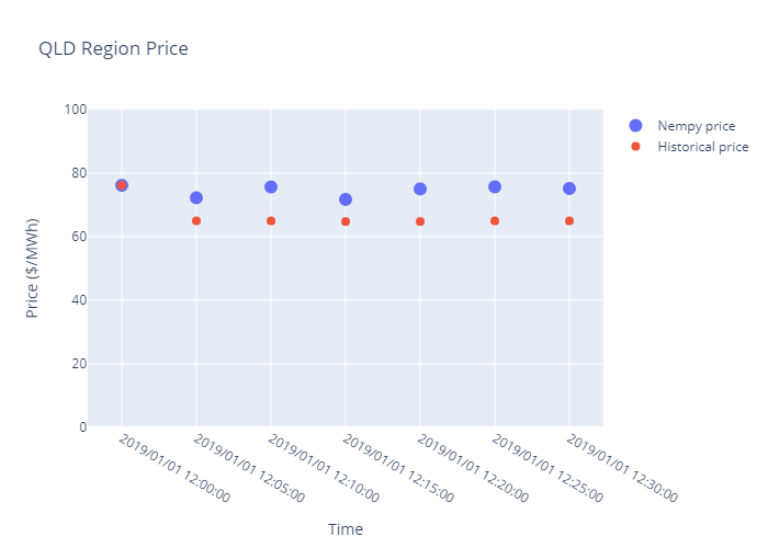
Results from example: for the QLD region a reasonable fit between modelled prices and historical prices is obtained.
Warning
Warning this script downloads approximately 8.5 GB of data from AEMO. The download_inputs flag can be set to false to stop the script re-downloading data for subsequent runs.
Note
This example also requires plotly >= 5.3.1, < 6.0.0 and kaleido == 0.2.1. Run pip install plotly==5.3.1 and pip install kaleido==0.2.1
  1# Notice:
  2# - This script downloads large volumes of historical market data from AEMO's nemweb
  3#   portal. The boolean on line 20 can be changed to prevent this happening repeatedly
  4#   once the data has been downloaded.
  5# - This example also requires plotly >= 5.3.1, < 6.0.0 and kaleido == 0.2.1
  6#   pip install plotly==5.3.1 and pip install kaleido==0.2.1
  7
  8import sqlite3
  9import pandas as pd
 10import plotly.graph_objects as go
 11from nempy import markets
 12from nempy.historical_inputs import loaders, mms_db, \
 13    xml_cache, units, demand, interconnectors
 14
 15con = sqlite3.connect('historical_mms.db')
 16mms_db_manager = mms_db.DBManager(connection=con)
 17
 18xml_cache_manager = xml_cache.XMLCacheManager('nemde_cache')
 19
 20# The second time this example is run on a machine this flag can
 21# be set to false to save downloading the data again.
 22download_inputs = False
 23
 24if download_inputs:
 25    # This requires approximately 5 GB of storage.
 26    mms_db_manager.populate(start_year=2019, start_month=1,
 27                            end_year=2019, end_month=1)
 28
 29    # This requires approximately 3.5 GB of storage.
 30    xml_cache_manager.populate_by_day(start_year=2019, start_month=1, start_day=1,
 31                                      end_year=2019, end_month=1, end_day=1)
 32
 33raw_inputs_loader = loaders.RawInputsLoader(
 34    nemde_xml_cache_manager=xml_cache_manager,
 35    market_management_system_database=mms_db_manager)
 36
 37# A list of intervals we want to recreate historical dispatch for.
 38dispatch_intervals = ['2019/01/01 12:00:00',
 39                      '2019/01/01 12:05:00',
 40                      '2019/01/01 12:10:00',
 41                      '2019/01/01 12:15:00',
 42                      '2019/01/01 12:20:00',
 43                      '2019/01/01 12:25:00',
 44                      '2019/01/01 12:30:00']
 45
 46# List for saving outputs to.
 47outputs = []
 48
 49# Create and dispatch the spot market for each dispatch interval.
 50for interval in dispatch_intervals:
 51    raw_inputs_loader.set_interval(interval)
 52    unit_inputs = units.UnitData(raw_inputs_loader)
 53    demand_inputs = demand.DemandData(raw_inputs_loader)
 54    interconnector_inputs = \
 55        interconnectors.InterconnectorData(raw_inputs_loader)
 56
 57    unit_info = unit_inputs.get_unit_info()
 58    market = markets.SpotMarket(market_regions=['QLD1', 'NSW1', 'VIC1',
 59                                                'SA1', 'TAS1'],
 60                                unit_info=unit_info)
 61
 62    volume_bids, price_bids = unit_inputs.get_processed_bids()
 63    market.set_unit_volume_bids(volume_bids)
 64    market.set_unit_price_bids(price_bids)
 65
 66    unit_bid_limit = unit_inputs.get_unit_bid_availability()
 67    market.set_unit_bid_capacity_constraints(unit_bid_limit)
 68
 69    unit_uigf_limit = unit_inputs.get_unit_uigf_limits()
 70    market.set_unconstrained_intermittent_generation_forecast_constraint(
 71        unit_uigf_limit)
 72
 73    regional_demand = demand_inputs.get_operational_demand()
 74    market.set_demand_constraints(regional_demand)
 75
 76    interconnectors_definitions = \
 77        interconnector_inputs.get_interconnector_definitions()
 78    loss_functions, interpolation_break_points = \
 79        interconnector_inputs.get_interconnector_loss_model()
 80    market.set_interconnectors(interconnectors_definitions)
 81    market.set_interconnector_losses(loss_functions,
 82                                     interpolation_break_points)
 83    market.dispatch()
 84
 85    # Save prices from this interval
 86    prices = market.get_energy_prices()
 87    prices['time'] = interval
 88
 89    # Getting historical prices for comparison. Note, ROP price, which is
 90    # the regional reference node price before the application of any
 91    # price scaling by AEMO, is used for comparison.
 92    historical_prices = mms_db_manager.DISPATCHPRICE.get_data(interval)
 93
 94    prices = pd.merge(prices, historical_prices,
 95                      left_on=['time', 'region'],
 96                      right_on=['SETTLEMENTDATE', 'REGIONID'])
 97
 98    outputs.append(
 99        prices.loc[:, ['time', 'region', 'price', 'ROP']])
100
101con.close()
102
103outputs = pd.concat(outputs)
104
105# Plot results for QLD market region.
106qld_prices = outputs[outputs['region'] == 'QLD1']
107
108fig = go.Figure()
109fig.add_trace(go.Scatter(x=qld_prices['time'], y=qld_prices['price'], name='Nempy price', mode='markers',
110                         marker_size=12, marker_symbol='circle'))
111fig.add_trace(go.Scatter(x=qld_prices['time'], y=qld_prices['ROP'], name='Historical price', mode='markers',
112                         marker_size=8))
113fig.update_xaxes(title="Time")
114fig.update_yaxes(title="Price ($/MWh)")
115fig.update_layout(yaxis_range=[0.0, 100.0], title="QLD Region Price")
116fig.write_image('energy_market_only_qld_prices.png')
117fig.show()
118
119print(outputs)
120#                   time region      price       ROP
121# 0  2019/01/01 12:00:00   NSW1  91.857666  91.87000
122# 1  2019/01/01 12:00:00   QLD1  76.180429  76.19066
123# 2  2019/01/01 12:00:00    SA1  85.126914  86.89938
124# 3  2019/01/01 12:00:00   TAS1  85.948523  89.70523
125# 4  2019/01/01 12:00:00   VIC1  83.250703  84.98410
126# 0  2019/01/01 12:05:00   NSW1  88.357224  91.87000
127# 1  2019/01/01 12:05:00   QLD1  72.255334  64.99000
128# 2  2019/01/01 12:05:00    SA1  82.417720  87.46213
129# 3  2019/01/01 12:05:00   TAS1  83.451561  90.08096
130# 4  2019/01/01 12:05:00   VIC1  80.621103  85.55555
131# 0  2019/01/01 12:10:00   NSW1  91.857666  91.87000
132# 1  2019/01/01 12:10:00   QLD1  75.665675  64.99000
133# 2  2019/01/01 12:10:00    SA1  85.680310  86.86809
134# 3  2019/01/01 12:10:00   TAS1  86.715499  89.87995
135# 4  2019/01/01 12:10:00   VIC1  83.774337  84.93569
136# 0  2019/01/01 12:15:00   NSW1  88.343034  91.87000
137# 1  2019/01/01 12:15:00   QLD1  71.746786  64.78003
138# 2  2019/01/01 12:15:00    SA1  82.379539  86.84407
139# 3  2019/01/01 12:15:00   TAS1  83.451561  89.48585
140# 4  2019/01/01 12:15:00   VIC1  80.621103  84.99034
141# 0  2019/01/01 12:20:00   NSW1  91.864122  91.87000
142# 1  2019/01/01 12:20:00   QLD1  75.052319  64.78003
143# 2  2019/01/01 12:20:00    SA1  85.722028  87.49564
144# 3  2019/01/01 12:20:00   TAS1  86.576848  90.28958
145# 4  2019/01/01 12:20:00   VIC1  83.859306  85.59438
146# 0  2019/01/01 12:25:00   NSW1  91.864122  91.87000
147# 1  2019/01/01 12:25:00   QLD1  75.696247  64.99000
148# 2  2019/01/01 12:25:00    SA1  85.746024  87.51983
149# 3  2019/01/01 12:25:00   TAS1  86.613642  90.38750
150# 4  2019/01/01 12:25:00   VIC1  83.894945  85.63046
151# 0  2019/01/01 12:30:00   NSW1  91.870167  91.87000
152# 1  2019/01/01 12:30:00   QLD1  75.188735  64.99000
153# 2  2019/01/01 12:30:00    SA1  85.694071  87.46153
154# 3  2019/01/01 12:30:00   TAS1  86.560602  90.09919
155# 4  2019/01/01 12:30:00   VIC1  83.843570  85.57286
7. Detailed recreation of historical dispatch with Basslink switch run
This example demonstrates using Nempy to recreate historical dispatch intervals by implementing an energy market using all the features of the Nempy market model, with inputs sourced from historical data published by AEMO. This example has been updated to include the use of functionality developed to enable modelling the Basslink switch run, which is new in Nempy version 2.0.0. Previously, Nempy relied on using the generic constraint RHS values reported with the NEMDE solution from what historically was the least cost case of the switch run. However, the new functionality allows the RHS values for each case of the switch run to be calculated by Nempy, and so for each case of switch run to be tested.
Warning
Warning this script downloads approximately 54 GB of data from AEMO. The download_inputs flag can be set to false to stop the script re-downloading data for subsequent runs.
  1# Notice:
  2# - This script downloads large volumes of historical market data (~54 GB) from AEMO's nemweb
  3#   portal. You can also reduce the data usage by restricting the time window given to the
  4#   xml_cache_manager and in the get_test_intervals function. The boolean on line 23 can
  5#   also be changed to prevent this happening repeatedly once the data has been downloaded.
  6
  7import sqlite3
  8from datetime import datetime, timedelta
  9import random
 10import pandas as pd
 11from nempy import markets
 12from nempy.historical_inputs import loaders, mms_db, \
 13    xml_cache, units, demand, interconnectors, constraints, rhs_calculator
 14from nempy.help_functions.helper_functions import update_rhs_values
 15
 16con = sqlite3.connect('D:/nempy_2024_07/historical_mms.db')
 17mms_db_manager = mms_db.DBManager(connection=con)
 18
 19xml_cache_manager = xml_cache.XMLCacheManager('D:/nempy_2024_07/xml_cache')
 20
 21# The second time this example is run on a machine this flag can
 22# be set to false to save downloading the data again.
 23download_inputs = True
 24
 25if download_inputs:
 26    # This requires approximately 4 GB of storage.
 27    mms_db_manager.populate(start_year=2024, start_month=7,
 28                            end_year=2024, end_month=7)
 29
 30    # This requires approximately 50 GB of storage.
 31    xml_cache_manager.populate_by_day(start_year=2024, start_month=7, start_day=1,
 32                                      end_year=2024, end_month=8, end_day=1)
 33
 34raw_inputs_loader = loaders.RawInputsLoader(
 35    nemde_xml_cache_manager=xml_cache_manager,
 36    market_management_system_database=mms_db_manager)
 37
 38
 39# A list of intervals we want to recreate historical dispatch for.
 40def get_test_intervals(number=100):
 41    start_time = datetime(year=2024, month=7, day=1, hour=0, minute=0)
 42    end_time = datetime(year=2024, month=8, day=1, hour=0, minute=0)
 43    difference = end_time - start_time
 44    difference_in_5_min_intervals = difference.days * 12 * 24
 45    random.seed(1)
 46    intervals = random.sample(range(1, difference_in_5_min_intervals), number)
 47    times = [start_time + timedelta(minutes=5 * i) for i in intervals]
 48    times_formatted = [t.isoformat().replace('T', ' ').replace('-', '/') for t in times]
 49    return times_formatted
 50
 51
 52# List for saving outputs to.
 53outputs = []
 54c = 0
 55# Create and dispatch the spot market for each dispatch interval.
 56for interval in get_test_intervals(number=100):
 57    c += 1
 58    print(str(c) + ' ' + str(interval))
 59    raw_inputs_loader.set_interval(interval)
 60    unit_inputs = units.UnitData(raw_inputs_loader)
 61    interconnector_inputs = interconnectors.InterconnectorData(raw_inputs_loader)
 62    constraint_inputs = constraints.ConstraintData(raw_inputs_loader)
 63    demand_inputs = demand.DemandData(raw_inputs_loader)
 64    rhs_calculation_engine = rhs_calculator.RHSCalc(xml_cache_manager)
 65
 66    unit_info = unit_inputs.get_unit_info()
 67    market = markets.SpotMarket(market_regions=['QLD1', 'NSW1', 'VIC1',
 68                                                'SA1', 'TAS1'],
 69                                unit_info=unit_info)
 70
 71    # Set bids
 72    volume_bids, price_bids = unit_inputs.get_processed_bids()
 73    market.set_unit_volume_bids(volume_bids)
 74    market.set_unit_price_bids(price_bids)
 75
 76    # Set bid in capacity limits
 77    unit_bid_limit = unit_inputs.get_unit_bid_availability()
 78    market.set_unit_bid_capacity_constraints(unit_bid_limit)
 79    cost = constraint_inputs.get_constraint_violation_prices()['unit_capacity']
 80    market.make_constraints_elastic('unit_bid_capacity', violation_cost=cost)
 81
 82    # Set limits provided by the unconstrained intermittent generation
 83    # forecasts. Primarily for wind and solar.
 84    unit_uigf_limit = unit_inputs.get_unit_uigf_limits()
 85    market.set_unconstrained_intermittent_generation_forecast_constraint(
 86        unit_uigf_limit)
 87    cost = constraint_inputs.get_constraint_violation_prices()['uigf']
 88    market.make_constraints_elastic('uigf_capacity', violation_cost=cost)
 89
 90    ramp_rates = unit_inputs.get_bid_ramp_rates()
 91    scada_ramp_rates = unit_inputs.get_scada_ramp_rates(inlude_initial_output=True)
 92    initial_fast_start_profiles = unit_inputs.get_fast_start_profiles_for_dispatch()
 93
 94    # Set unit ramp rates.
 95    def set_ramp_rates(run_type, fsp):
 96        if run_type == "fast_start_first_run":
 97            fsp = fsp.loc[:, ['unit', 'current_mode']]
 98        else:
 99            fsp = fsp.loc[:, ['unit', 'end_mode', 'time_since_end_of_mode_two', 'min_loading']]
100        cost = constraint_inputs.get_constraint_violation_prices()['ramp_rate']
101        market.set_unit_ramp_rate_constraints(
102            ramp_rates,
103            scada_ramp_rates.loc[:, ['unit', 'scada_ramp_up_rate', 'scada_ramp_down_rate']],
104            fsp,
105            run_type=run_type, violation_cost=cost
106        )
107        cost = constraint_inputs.get_constraint_violation_prices()['fcas_profile']
108        market.set_joint_ramping_constraints_reg(
109            scada_ramp_rates, fsp, run_type=run_type, violation_cost=cost
110        )
111
112
113    set_ramp_rates('fast_start_first_run', initial_fast_start_profiles)
114
115    # Set unit FCAS trapezium constraints.
116    unit_inputs.add_fcas_trapezium_constraints()
117    cost = constraint_inputs.get_constraint_violation_prices()['fcas_max_avail']
118    fcas_availability = unit_inputs.get_fcas_max_availability()
119    market.set_fcas_max_availability(fcas_availability, violation_cost=cost)
120    cost = constraint_inputs.get_constraint_violation_prices()['fcas_profile']
121    regulation_trapeziums = unit_inputs.get_fcas_regulation_trapeziums()
122    market.set_energy_and_regulation_capacity_constraints(regulation_trapeziums, violation_cost=cost)
123    contingency_trapeziums = unit_inputs.get_contingency_services()
124    market.set_joint_capacity_constraints(contingency_trapeziums, violation_cost=cost)
125
126    # Set interconnector definitions, limits and loss models.
127    interconnectors_definitions = \
128        interconnector_inputs.get_interconnector_definitions()
129    loss_functions, interpolation_break_points = \
130        interconnector_inputs.get_interconnector_loss_model()
131    market.set_interconnectors(interconnectors_definitions)
132    market.set_interconnector_losses(loss_functions,
133                                     interpolation_break_points)
134
135    # Calculate rhs constraint values that depend on the basslink frequency controller from scratch so there is
136    # consistency between the basslink switch runs.
137    # Find the constraints that need to be calculated because they depend on the frequency controller status.
138    constraints_to_update = (
139        rhs_calculation_engine.get_rhs_constraint_equations_that_depend_value('BL_FREQ_ONSTATUS', 'W'))
140    initial_bl_freq_onstatus = rhs_calculation_engine.scada_data['W']['BL_FREQ_ONSTATUS'][0]['@Value']
141    # Calculate new rhs values for the constraints that need updating.
142    new_rhs_values = rhs_calculation_engine.compute_constraint_rhs(constraints_to_update)
143
144    # Add generic constraints and FCAS market constraints.
145    fcas_requirements = constraint_inputs.get_fcas_requirements()
146    fcas_requirements = update_rhs_values(fcas_requirements, new_rhs_values)
147    cost = constraint_inputs.get_violation_costs()
148    market.set_fcas_requirements_constraints(fcas_requirements, violation_cost=cost)
149    generic_rhs = constraint_inputs.get_rhs_and_type_excluding_regional_fcas_constraints()
150    generic_rhs = update_rhs_values(generic_rhs, new_rhs_values)
151    market.set_generic_constraints(generic_rhs, violation_cost=cost)
152
153    unit_generic_lhs = constraint_inputs.get_unit_lhs()
154    market.link_units_to_generic_constraints(unit_generic_lhs)
155    interconnector_generic_lhs = constraint_inputs.get_interconnector_lhs()
156    market.link_interconnectors_to_generic_constraints(
157        interconnector_generic_lhs)
158
159    # Set the operational demand to be met by dispatch.
160    regional_demand = demand_inputs.get_operational_demand()
161    cost = constraint_inputs.get_constraint_violation_prices()['regional_demand']
162    market.set_demand_constraints(regional_demand, violation_cost=cost)
163
164    # Set tiebreak constraint to equalise dispatch of equally priced bids.
165    cost = constraint_inputs.get_constraint_violation_prices()['tiebreak']
166    market.set_tie_break_constraints(cost)
167
168    # Get unit dispatch without fast start constraints and use it to
169    # make fast start unit commitment decisions.
170    market.dispatch()
171    dispatch = market.get_unit_dispatch()
172    fast_start_profiles = unit_inputs.get_fast_start_profiles_for_dispatch(dispatch)
173    set_ramp_rates('fast_start_second_run', fast_start_profiles)
174    cost = constraint_inputs.get_constraint_violation_prices()['fast_start']
175    cols = ['unit', 'end_mode', 'time_in_end_mode', 'mode_two_length',
176            'mode_four_length', 'min_loading']
177    fsp = fast_start_profiles.loc[:, cols]
178    market.set_fast_start_constraints(fsp, violation_cost=cost)
179
180    # First run of Basslink switch runs
181    market.dispatch()  # First dispatch without allowing over constrained dispatch re-run to get objective function.
182    objective_value_run_one = market.objective_value
183    if constraint_inputs.is_over_constrained_dispatch_rerun():
184        market.dispatch(allow_over_constrained_dispatch_re_run=True,
185                        energy_market_floor_price=-1000.0,
186                        energy_market_ceiling_price=17500.0,
187                        fcas_market_ceiling_price=1000.0)
188    prices_run_one = market.get_energy_prices()  # If this is the lowest cost run these will be the market prices.
189
190    # Re-run dispatch with Basslink Frequency controller off.
191    # Set frequency controller to off in rhs calculations
192    rhs_calculation_engine.update_spd_id_value('BL_FREQ_ONSTATUS', 'W', '0')
193    new_bl_freq_onstatus = rhs_calculation_engine.scada_data['W']['BL_FREQ_ONSTATUS'][0]['@Value']
194    # Find the constraints that need to be updated because they depend on the frequency controller status.
195    constraints_to_update = (
196        rhs_calculation_engine.get_rhs_constraint_equations_that_depend_value('BL_FREQ_ONSTATUS', 'W'))
197    # Calculate new rhs values for the constraints that need updating.
198    new_rhs_values = rhs_calculation_engine.compute_constraint_rhs(constraints_to_update)
199    # Update the constraints in the market.
200    fcas_requirements = update_rhs_values(fcas_requirements, new_rhs_values)
201    cost = constraint_inputs.get_violation_costs()
202    market.set_fcas_requirements_constraints(fcas_requirements, violation_cost=cost)
203    generic_rhs = update_rhs_values(generic_rhs, new_rhs_values)
204    market.set_generic_constraints(generic_rhs, violation_cost=cost)
205
206    # Reset ramp rate constraints for first run of second Basslink switchrun
207    set_ramp_rates('fast_start_first_run', initial_fast_start_profiles)
208
209    # Get unit dispatch without fast start constraints and use it to
210    # make fast start unit commitment decisions.
211    market.remove_fast_start_constraints()
212    market.dispatch()
213    dispatch = market.get_unit_dispatch()
214    fast_start_profiles = unit_inputs.get_fast_start_profiles_for_dispatch(dispatch)
215    set_ramp_rates('fast_start_second_run', fast_start_profiles)
216    cost = constraint_inputs.get_constraint_violation_prices()['fast_start']
217    cols = ['unit', 'end_mode', 'time_in_end_mode', 'mode_two_length',
218            'mode_four_length', 'min_loading']
219    fsp = fast_start_profiles.loc[:, cols]
220    market.set_fast_start_constraints(fsp, violation_cost=cost)
221
222    market.dispatch()  # First dispatch without allowing over constrained dispatch re-run to get objective function.
223    objective_value_run_two = market.objective_value
224    if constraint_inputs.is_over_constrained_dispatch_rerun():
225        market.dispatch(allow_over_constrained_dispatch_re_run=True,
226                        energy_market_floor_price=-1000.0,
227                        energy_market_ceiling_price=17500.0,
228                        fcas_market_ceiling_price=1000.0)
229    prices_run_two = market.get_energy_prices()  # If this is the lowest cost run these will be the market prices.
230
231    prices_run_one['time'] = interval
232    prices_run_two['time'] = interval
233
234    # Getting historical prices for comparison. Note, ROP price, which is
235    # the regional reference node price before the application of any
236    # price scaling by AEMO, is used for comparison.
237    historical_prices = mms_db_manager.DISPATCHPRICE.get_data(interval)
238
239    # The prices from the run with the lowest objective function value are used.
240    if objective_value_run_one < objective_value_run_two:
241        prices = prices_run_one
242    else:
243        prices = prices_run_two
244
245    prices['time'] = interval
246    prices = pd.merge(prices, historical_prices,
247                      left_on=['time', 'region'],
248                      right_on=['SETTLEMENTDATE', 'REGIONID'])
249
250    outputs.append(prices)
251
252con.close()
253
254outputs = pd.concat(outputs)
255
256outputs['error'] = outputs['price'] - outputs['ROP']
257
258print('\n Summary of error in energy price volume weighted average price. \n'
259      'Comparison is against ROP, the price prior to \n'
260      'any post dispatch adjustments, scaling, capping etc.')
261print('Mean price error: {}'.format(outputs['error'].mean()))
262print('Median price error: {}'.format(outputs['error'].quantile(0.5)))
263print('5% percentile price error: {}'.format(outputs['error'].quantile(0.05)))
264print('95% percentile price error: {}'.format(outputs['error'].quantile(0.95)))
265
266# Summary of error in energy price volume weighted average price.
267# Comparison is against ROP, the price prior to
268# any post dispatch adjustments, scaling, capping etc.
269# Mean price error: 0.15175124971435794
270# Median price error: 0.0
271# 5% percentile price error: -0.2187800690807549
272# 95% percentile price error: 0.027599033294391225
273
7. Recreation of historical dispatch without Basslink switchrun
This example demonstrates using Nempy to recreate historical dispatch intervals by implementing an energy market using all the features of the Nempy market model, except the Basslink switch run, with inputs sourced from historical data published by AEMO. The main reason not to include Basslink switch run is to speed up runtime. Note each interval is dispatched as a standalone simulation and the results from one dispatch interval are not carried over to be the initial conditions of the next interval, rather the historical initial conditions are always used.
Warning
Warning this script downloads approximately 54 GB of data from AEMO. The download_inputs flag can be set to false to stop the script re-downloading data for subsequent runs.
  1# Notice:
  2# - This script downloads large volumes of historical market data (~54 GB) from AEMO's nemweb
  3#   portal. You can also reduce the data usage by restricting the time window given to the
  4#   xml_cache_manager and in the get_test_intervals function. The boolean on line 22 can
  5#   also be changed to prevent this happening repeatedly once the data has been downloaded.
  6
  7import sqlite3
  8from datetime import datetime, timedelta
  9import random
 10import pandas as pd
 11from nempy import markets
 12from nempy.historical_inputs import loaders, mms_db, \
 13    xml_cache, units, demand, interconnectors, constraints
 14
 15con = sqlite3.connect('D:/nempy_2024_07/historical_mms.db')
 16mms_db_manager = mms_db.DBManager(connection=con)
 17
 18xml_cache_manager = xml_cache.XMLCacheManager('D:/nempy_2024_07/xml_cache')
 19
 20# The second time this example is run on a machine this flag can
 21# be set to false to save downloading the data again.
 22download_inputs = True
 23
 24if download_inputs:
 25    # This requires approximately 4 GB of storage.
 26    mms_db_manager.populate(start_year=2024, start_month=7,
 27                            end_year=2024, end_month=7)
 28
 29    # This requires approximately 50 GB of storage.
 30    xml_cache_manager.populate_by_day(start_year=2024, start_month=7, start_day=1,
 31                                      end_year=2024, end_month=8, end_day=1)
 32
 33raw_inputs_loader = loaders.RawInputsLoader(
 34    nemde_xml_cache_manager=xml_cache_manager,
 35    market_management_system_database=mms_db_manager)
 36
 37
 38# A list of intervals we want to recreate historical dispatch for.
 39def get_test_intervals(number=100):
 40    start_time = datetime(year=2024, month=7, day=1, hour=0, minute=0)
 41    end_time = datetime(year=2024, month=8, day=1, hour=0, minute=0)
 42    difference = end_time - start_time
 43    difference_in_5_min_intervals = difference.days * 12 * 24
 44    random.seed(1)
 45    intervals = random.sample(range(1, difference_in_5_min_intervals), number)
 46    times = [start_time + timedelta(minutes=5 * i) for i in intervals]
 47    times_formatted = [t.isoformat().replace('T', ' ').replace('-', '/') for t in times]
 48    return times_formatted
 49
 50
 51# List for saving outputs to.
 52outputs = []
 53c = 0
 54# Create and dispatch the spot market for each dispatch interval.
 55for interval in get_test_intervals(number=100):
 56
 57    c += 1
 58    print(str(c) + ' ' + str(interval))
 59    raw_inputs_loader.set_interval(interval)
 60    unit_inputs = units.UnitData(raw_inputs_loader)
 61    interconnector_inputs = interconnectors.InterconnectorData(raw_inputs_loader)
 62    constraint_inputs = constraints.ConstraintData(raw_inputs_loader)
 63    demand_inputs = demand.DemandData(raw_inputs_loader)
 64
 65    unit_info = unit_inputs.get_unit_info()
 66    market = markets.SpotMarket(market_regions=['QLD1', 'NSW1', 'VIC1',
 67                                                'SA1', 'TAS1'],
 68                                unit_info=unit_info)
 69
 70    # Set bids
 71    volume_bids, price_bids = unit_inputs.get_processed_bids()
 72    market.set_unit_volume_bids(volume_bids)
 73    market.set_unit_price_bids(price_bids)
 74
 75    # Set bid in capacity limits
 76    unit_bid_limit = unit_inputs.get_unit_bid_availability()
 77    cost = constraint_inputs.get_constraint_violation_prices()['unit_capacity']
 78    market.set_unit_bid_capacity_constraints(unit_bid_limit, violation_cost=cost)
 79
 80    # Set limits provided by the unconstrained intermittent generation
 81    # forecasts. Primarily for wind and solar.
 82    unit_uigf_limit = unit_inputs.get_unit_uigf_limits()
 83    cost = constraint_inputs.get_constraint_violation_prices()['uigf']
 84    market.set_unconstrained_intermittent_generation_forecast_constraint(
 85        unit_uigf_limit, violation_cost=cost
 86    )
 87
 88    # Set unit ramp rates.
 89    ramp_rates = unit_inputs.get_bid_ramp_rates()
 90    scada_ramp_rates = unit_inputs.get_scada_ramp_rates()
 91    fast_start_profiles = unit_inputs.get_fast_start_profiles_for_dispatch()
 92    cost = constraint_inputs.get_constraint_violation_prices()['ramp_rate']
 93    market.set_unit_ramp_rate_constraints(
 94        ramp_rates, scada_ramp_rates, fast_start_profiles,
 95        run_type="fast_start_first_run", violation_cost=cost
 96    )
 97
 98    # Set unit FCAS trapezium constraints.
 99    unit_inputs.add_fcas_trapezium_constraints()
100    cost = constraint_inputs.get_constraint_violation_prices()['fcas_max_avail']
101    fcas_availability = unit_inputs.get_fcas_max_availability()
102    market.set_fcas_max_availability(fcas_availability, violation_cost=cost)
103    cost = constraint_inputs.get_constraint_violation_prices()['fcas_profile']
104    regulation_trapeziums = unit_inputs.get_fcas_regulation_trapeziums()
105    market.set_energy_and_regulation_capacity_constraints(regulation_trapeziums,
106                                                          violation_cost=cost)
107    scada_ramp_rates = unit_inputs.get_scada_ramp_rates(inlude_initial_output=True)
108    market.set_joint_ramping_constraints_reg(
109        scada_ramp_rates, fast_start_profiles, run_type="fast_start_first_run",
110        violation_cost=cost
111    )
112    contingency_trapeziums = unit_inputs.get_contingency_services()
113    market.set_joint_capacity_constraints(contingency_trapeziums, violation_cost=cost)
114
115    # Set interconnector definitions, limits and loss models.
116    interconnectors_definitions = \
117        interconnector_inputs.get_interconnector_definitions()
118    loss_functions, interpolation_break_points = \
119        interconnector_inputs.get_interconnector_loss_model()
120    market.set_interconnectors(interconnectors_definitions)
121    market.set_interconnector_losses(loss_functions,
122                                     interpolation_break_points)
123
124    # Add generic constraints and FCAS market constraints.
125    fcas_requirements = constraint_inputs.get_fcas_requirements()
126    cost = constraint_inputs.get_violation_costs()
127    market.set_fcas_requirements_constraints(fcas_requirements, violation_cost=cost)
128    generic_rhs = constraint_inputs.get_rhs_and_type_excluding_regional_fcas_constraints()
129    market.set_generic_constraints(generic_rhs, violation_cost=cost)
130    unit_generic_lhs = constraint_inputs.get_unit_lhs()
131    market.link_units_to_generic_constraints(unit_generic_lhs)
132    interconnector_generic_lhs = constraint_inputs.get_interconnector_lhs()
133    market.link_interconnectors_to_generic_constraints(interconnector_generic_lhs)
134
135    # Set the operational demand to be met by dispatch.
136    regional_demand = demand_inputs.get_operational_demand()
137    cost = constraint_inputs.get_constraint_violation_prices()['regional_demand']
138    market.set_demand_constraints(regional_demand, violation_cost=cost)
139
140    # Set tiebreak constraint to equalise dispatch of equally priced bids.
141    cost = constraint_inputs.get_constraint_violation_prices()['tiebreak']
142    market.set_tie_break_constraints(cost)
143
144    # Get unit dispatch without fast start constraints and use it to
145    # make fast start unit commitment decisions.
146    market.dispatch()
147    dispatch = market.get_unit_dispatch()
148
149    cost = constraint_inputs.get_constraint_violation_prices()['fast_start']
150    fast_start_profiles = unit_inputs.get_fast_start_profiles_for_dispatch(dispatch)
151    cols = ['unit', 'end_mode', 'time_in_end_mode', 'mode_two_length',
152            'mode_four_length', 'min_loading']
153    fsp = fast_start_profiles.loc[:, cols]
154    market.set_fast_start_constraints(fsp, violation_cost=cost)
155
156    ramp_rates = unit_inputs.get_bid_ramp_rates()
157    scada_ramp_rates = unit_inputs.get_scada_ramp_rates()
158    cols = ['unit', 'end_mode', 'time_since_end_of_mode_two', 'min_loading']
159    fsp = fast_start_profiles.loc[:, cols]
160    cost = constraint_inputs.get_constraint_violation_prices()['ramp_rate']
161    market.set_unit_ramp_rate_constraints(
162        ramp_rates, scada_ramp_rates, fsp,
163        run_type="fast_start_second_run", violation_cost=cost
164    )
165    cost = constraint_inputs.get_constraint_violation_prices()['fcas_profile']
166    scada_ramp_rates = unit_inputs.get_scada_ramp_rates(inlude_initial_output=True)
167    market.set_joint_ramping_constraints_reg(
168        scada_ramp_rates, fsp, run_type="fast_start_second_run", violation_cost=cost
169    )
170
171    # If AEMO historically used the over constrained dispatch rerun
172    # process then allow it to be used in dispatch. This is needed
173    # because sometimes the conditions for over constrained dispatch
174    # are present but the rerun process isn't used.
175    if constraint_inputs.is_over_constrained_dispatch_rerun():
176        market.dispatch(allow_over_constrained_dispatch_re_run=True,
177                        energy_market_floor_price=-1000.0,
178                        energy_market_ceiling_price=17500.0,
179                        fcas_market_ceiling_price=1000.0)
180    else:
181        # The market price ceiling and floor are not needed here
182        # because they are only used for the over constrained
183        # dispatch rerun process.
184        market.dispatch(allow_over_constrained_dispatch_re_run=False)
185
186    # Save prices from this interval
187    prices = market.get_energy_prices()
188    prices['time'] = interval
189
190    # Getting historical prices for comparison. Note, ROP price, which is
191    # the regional reference node price before the application of any
192    # price scaling by AEMO, is used for comparison.
193    historical_prices = mms_db_manager.DISPATCHPRICE.get_data(interval)
194
195    prices = pd.merge(prices, historical_prices,
196                      left_on=['time', 'region'],
197                      right_on=['SETTLEMENTDATE', 'REGIONID'])
198
199    outputs.append(
200        prices.loc[:, ['time', 'region', 'price', 'ROP']])
201
202con.close()
203
204outputs = pd.concat(outputs)
205
206outputs['error'] = outputs['price'] - outputs['ROP']
207
208outputs.to_csv("bdu_prices.csv")
209
210print('\n Summary of error in energy price volume weighted average price. \n'
211      'Comparison is against ROP, the price prior to \n'
212      'any post dispatch adjustments, scaling, capping etc.')
213print('Mean price error: {}'.format(outputs['error'].mean()))
214print('Median price error: {}'.format(outputs['error'].quantile(0.5)))
215print('5% percentile price error: {}'.format(outputs['error'].quantile(0.05)))
216print('95% percentile price error: {}'.format(outputs['error'].quantile(0.95)))
217
218# Summary of error in energy price volume weighted average price.
219# Comparison is against ROP, the price prior to
220# any post dispatch adjustments, scaling, capping etc.
221# Mean price error: 0.13818277307210394
222# Median price error: 0.0
223# 5% percentile price error: -0.13335830516772942
224# 95% percentile price error: 0.013533539900288811
8. Time sequential recreation of historical dispatch
This example demonstrates using Nempy to recreate historical dispatch in a dynamic or time sequential manner, this means the outputs of one interval become the initial conditions for the next dispatch interval. Note, currently there is not the infrastructure in place to include features such as generic constraints in the time sequential model as the rhs values of many constraints would need to be re-calculated based on the dynamic system state. Similarly, using historical bids in this example is some what problematic as participants also dynamically change their bids based on market conditions. However, for the sake of demonstrating how Nempy can be used to create time sequential models, historical bids are used in this example.
Warning
Warning this script downloads approximately 8.5 GB of data from AEMO. The download_inputs flag can be set to false to stop the script re-downloading data for subsequent runs.
  1# Notice:
  2# - This script downloads large volumes of historical market data from AEMO's nemweb
  3#   portal. The boolean on line 20 can be changed to prevent this happening repeatedly
  4#   once the data has been downloaded.
  5# - This example also requires plotly >= 5.3.1, < 6.0.0 and kaleido == 0.2.1
  6#   pip install plotly==5.3.1 and pip install kaleido==0.2.1
  7
  8import sqlite3
  9import pandas as pd
 10from nempy import markets, time_sequential
 11from nempy.historical_inputs import loaders, mms_db, \
 12    xml_cache, units, demand, interconnectors, constraints
 13
 14con = sqlite3.connect('market_management_system.db')
 15mms_db_manager = mms_db.DBManager(connection=con)
 16
 17xml_cache_manager = xml_cache.XMLCacheManager('cache_directory')
 18
 19# The second time this example is run on a machine this flag can
 20# be set to false to save downloading the data again.
 21download_inputs = True
 22
 23if download_inputs:
 24    # This requires approximately 5 GB of storage.
 25    mms_db_manager.populate(start_year=2019, start_month=1,
 26                            end_year=2019, end_month=1)
 27
 28    # This requires approximately 3.5 GB of storage.
 29    xml_cache_manager.populate_by_day(start_year=2019, start_month=1, start_day=1,
 30                                      end_year=2019, end_month=1, end_day=1)
 31
 32raw_inputs_loader = loaders.RawInputsLoader(
 33    nemde_xml_cache_manager=xml_cache_manager,
 34    market_management_system_database=mms_db_manager)
 35
 36# A list of intervals we want to recreate historical dispatch for.
 37dispatch_intervals = ['2019/01/01 12:00:00',
 38                      '2019/01/01 12:05:00',
 39                      '2019/01/01 12:10:00',
 40                      '2019/01/01 12:15:00',
 41                      '2019/01/01 12:20:00',
 42                      '2019/01/01 12:25:00',
 43                      '2019/01/01 12:30:00']
 44
 45# List for saving outputs to.
 46outputs = []
 47
 48unit_dispatch = None
 49from time import time
 50
 51t0 = time()
 52# Create and dispatch the spot market for each dispatch interval.
 53for interval in dispatch_intervals:
 54    print(interval)
 55    raw_inputs_loader.set_interval(interval)
 56    unit_inputs = units.UnitData(raw_inputs_loader)
 57    demand_inputs = demand.DemandData(raw_inputs_loader)
 58    interconnector_inputs = \
 59        interconnectors.InterconnectorData(raw_inputs_loader)
 60    constraint_inputs = \
 61        constraints.ConstraintData(raw_inputs_loader)
 62
 63    unit_info = unit_inputs.get_unit_info()
 64    market = markets.SpotMarket(market_regions=['QLD1', 'NSW1', 'VIC1',
 65                                                'SA1', 'TAS1'],
 66                                unit_info=unit_info)
 67
 68    volume_bids, price_bids = unit_inputs.get_processed_bids()
 69    market.set_unit_volume_bids(volume_bids)
 70    market.set_unit_price_bids(price_bids)
 71
 72    violation_cost = \
 73        constraint_inputs.get_constraint_violation_prices()['unit_capacity']
 74    unit_bid_limit = unit_inputs.get_unit_bid_availability()
 75    market.set_unit_bid_capacity_constraints(unit_bid_limit, violation_cost)
 76
 77    unit_uigf_limit = unit_inputs.get_unit_uigf_limits()
 78    market.set_unconstrained_intermittent_generation_forecast_constraint(
 79        unit_uigf_limit, violation_cost)
 80
 81    ramp_rates = unit_inputs.get_bid_ramp_rates()
 82
 83    # This is the part that makes it time sequential.
 84    if unit_dispatch is None:
 85        # For the first dispatch interval we use historical values
 86        # as initial conditions.
 87        historical_dispatch = unit_inputs.get_initial_unit_output()
 88        ramp_rates = time_sequential.create_seed_ramp_rate_parameters(
 89            historical_dispatch, ramp_rates)
 90    else:
 91        # For subsequent dispatch intervals we use the output levels
 92        # determined by the last dispatch as the new initial conditions
 93        ramp_rates = time_sequential.construct_ramp_rate_parameters(
 94            unit_dispatch, ramp_rates)
 95
 96    market.set_unit_ramp_rate_constraints(ramp_rates, violation_cost)
 97
 98    regional_demand = demand_inputs.get_operational_demand()
 99    market.set_demand_constraints(regional_demand)
100
101    interconnectors_definitions = \
102        interconnector_inputs.get_interconnector_definitions()
103    loss_functions, interpolation_break_points = \
104        interconnector_inputs.get_interconnector_loss_model()
105    market.set_interconnectors(interconnectors_definitions)
106    market.set_interconnector_losses(loss_functions,
107                                     interpolation_break_points)
108    market.dispatch()
109
110    # Save prices from this interval
111    prices = market.get_energy_prices()
112    prices['time'] = interval
113    outputs.append(prices.loc[:, ['time', 'region', 'price']])
114
115    unit_dispatch = market.get_unit_dispatch()
116
117print("Run time per interval {}".format((time()-t0)/len(dispatch_intervals)))
118con.close()
119print(pd.concat(outputs))
120#                   time region      price
121# 0  2019/01/01 12:00:00   NSW1  91.857666
122# 1  2019/01/01 12:00:00   QLD1  76.716642
123# 2  2019/01/01 12:00:00    SA1  85.126914
124# 3  2019/01/01 12:00:00   TAS1  86.173481
125# 4  2019/01/01 12:00:00   VIC1  83.250703
126# 0  2019/01/01 12:05:00   NSW1  88.357224
127# 1  2019/01/01 12:05:00   QLD1  72.255334
128# 2  2019/01/01 12:05:00    SA1  82.417720
129# 3  2019/01/01 12:05:00   TAS1  83.451561
130# 4  2019/01/01 12:05:00   VIC1  80.621103
131# 0  2019/01/01 12:10:00   NSW1  91.857666
132# 1  2019/01/01 12:10:00   QLD1  75.665675
133# 2  2019/01/01 12:10:00    SA1  85.680310
134# 3  2019/01/01 12:10:00   TAS1  86.715499
135# 4  2019/01/01 12:10:00   VIC1  83.774337
136# 0  2019/01/01 12:15:00   NSW1  88.113012
137# 1  2019/01/01 12:15:00   QLD1  71.559977
138# 2  2019/01/01 12:15:00    SA1  82.165045
139# 3  2019/01/01 12:15:00   TAS1  83.451561
140# 4  2019/01/01 12:15:00   VIC1  80.411187
141# 0  2019/01/01 12:20:00   NSW1  91.864122
142# 1  2019/01/01 12:20:00   QLD1  75.052319
143# 2  2019/01/01 12:20:00    SA1  85.722028
144# 3  2019/01/01 12:20:00   TAS1  86.576848
145# 4  2019/01/01 12:20:00   VIC1  83.859306
146# 0  2019/01/01 12:25:00   NSW1  91.864122
147# 1  2019/01/01 12:25:00   QLD1  75.696247
148# 2  2019/01/01 12:25:00    SA1  85.746024
149# 3  2019/01/01 12:25:00   TAS1  86.613642
150# 4  2019/01/01 12:25:00   VIC1  83.894945
151# 0  2019/01/01 12:30:00   NSW1  91.870167
152# 1  2019/01/01 12:30:00   QLD1  75.188735
153# 2  2019/01/01 12:30:00    SA1  85.694071
154# 3  2019/01/01 12:30:00   TAS1  86.560602
155# 4  2019/01/01 12:30:00   VIC1  83.843570
10. Nempy performance on older data (Jan 2013, without Basslink switch run)
This example demonstrates using Nempy to recreate historical dispatch intervals by implementing an energy market using all the features of the Nempy market model, with inputs sourced from historical data published by AEMO. A set of 100 random dispatch intervals from January 2015 are dispatched and compared to historical results to see how well Nempy performs for replicating older versions of the NEM’s dispatch procedure. Comparison is against ROP, the region price prior to any post dispatch adjustments, scaling, capping etc.
Summary of results:
Warning
Warning this script downloads approximately 54 GB of data from AEMO. The download_inputs flag can be set to false to stop the script re-downloading data for subsequent runs.
  1# Notice:
  2# - This script downloads large volumes of historical market data (~54 GB) from AEMO's nemweb
  3#   portal. You can also reduce the data usage by restricting the time window given to the
  4#   xml_cache_manager and in the get_test_intervals function. The boolean on line 22 can
  5#   also be changed to prevent this happening repeatedly once the data has been downloaded.
  6
  7import sqlite3
  8from datetime import datetime, timedelta
  9import random
 10import pandas as pd
 11from nempy import markets
 12from nempy.historical_inputs import loaders, mms_db, \
 13    xml_cache, units, demand, interconnectors, constraints
 14
 15con = sqlite3.connect('D:/nempy_2013/historical_mms.db')
 16mms_db_manager = mms_db.DBManager(connection=con)
 17
 18xml_cache_manager = xml_cache.XMLCacheManager('D:/nempy_2013/xml_cache')
 19
 20# The second time this example is run on a machine this flag can
 21# be set to false to save downloading the data again.
 22download_inputs = True
 23
 24if download_inputs:
 25    # This requires approximately 4 GB of storage.
 26    mms_db_manager.populate(start_year=2013, start_month=1,
 27                            end_year=2013, end_month=1)
 28
 29    # This requires approximately 50 GB of storage.
 30    xml_cache_manager.populate_by_day(start_year=2013, start_month=1, start_day=1,
 31                                      end_year=2013, end_month=2, end_day=1)
 32
 33raw_inputs_loader = loaders.RawInputsLoader(
 34    nemde_xml_cache_manager=xml_cache_manager,
 35    market_management_system_database=mms_db_manager)
 36
 37
 38# A list of intervals we want to recreate historical dispatch for.
 39def get_test_intervals(number=100):
 40    start_time = datetime(year=2013, month=1, day=1, hour=0, minute=0)
 41    end_time = datetime(year=2013, month=1, day=31, hour=0, minute=0)
 42    difference = end_time - start_time
 43    difference_in_5_min_intervals = difference.days * 12 * 24
 44    random.seed(1)
 45    intervals = random.sample(range(1, difference_in_5_min_intervals), number)
 46    times = [start_time + timedelta(minutes=5 * i) for i in intervals]
 47    times_formatted = [t.isoformat().replace('T', ' ').replace('-', '/') for t in times]
 48    return times_formatted
 49
 50
 51# List for saving outputs to.
 52outputs = []
 53c = 0
 54# Create and dispatch the spot market for each dispatch interval.
 55for interval in get_test_intervals(number=100):
 56
 57    c += 1
 58    print(str(c) + ' ' + str(interval))
 59    raw_inputs_loader.set_interval(interval)
 60    unit_inputs = units.UnitData(raw_inputs_loader)
 61    interconnector_inputs = interconnectors.InterconnectorData(raw_inputs_loader)
 62    constraint_inputs = constraints.ConstraintData(raw_inputs_loader)
 63    demand_inputs = demand.DemandData(raw_inputs_loader)
 64
 65    unit_info = unit_inputs.get_unit_info()
 66    market = markets.SpotMarket(market_regions=['QLD1', 'NSW1', 'VIC1',
 67                                                'SA1', 'TAS1'],
 68                                unit_info=unit_info)
 69
 70    # Set bids
 71    volume_bids, price_bids = unit_inputs.get_processed_bids()
 72    market.set_unit_volume_bids(volume_bids)
 73    market.set_unit_price_bids(price_bids)
 74
 75    # Set bid in capacity limits
 76    unit_bid_limit = unit_inputs.get_unit_bid_availability()
 77    cost = constraint_inputs.get_constraint_violation_prices()['unit_capacity']
 78    market.set_unit_bid_capacity_constraints(unit_bid_limit, violation_cost=cost)
 79
 80    # Set limits provided by the unconstrained intermittent generation
 81    # forecasts. Primarily for wind and solar.
 82    unit_uigf_limit = unit_inputs.get_unit_uigf_limits()
 83    cost = constraint_inputs.get_constraint_violation_prices()['uigf']
 84    market.set_unconstrained_intermittent_generation_forecast_constraint(
 85        unit_uigf_limit, violation_cost=cost
 86    )
 87
 88    # Set unit ramp rates.
 89    ramp_rates = unit_inputs.get_bid_ramp_rates()
 90    scada_ramp_rates = unit_inputs.get_scada_ramp_rates()
 91    fast_start_profiles = unit_inputs.get_fast_start_profiles_for_dispatch()
 92    cost = constraint_inputs.get_constraint_violation_prices()['ramp_rate']
 93    market.set_unit_ramp_rate_constraints(
 94        ramp_rates, scada_ramp_rates, fast_start_profiles,
 95        run_type="fast_start_first_run", violation_cost=cost
 96    )
 97
 98    # Set unit FCAS trapezium constraints.
 99    unit_inputs.add_fcas_trapezium_constraints()
100    cost = constraint_inputs.get_constraint_violation_prices()['fcas_max_avail']
101    fcas_availability = unit_inputs.get_fcas_max_availability()
102    market.set_fcas_max_availability(fcas_availability, violation_cost=cost)
103    cost = constraint_inputs.get_constraint_violation_prices()['fcas_profile']
104    regulation_trapeziums = unit_inputs.get_fcas_regulation_trapeziums()
105    market.set_energy_and_regulation_capacity_constraints(regulation_trapeziums,
106                                                          violation_cost=cost)
107    scada_ramp_rates = unit_inputs.get_scada_ramp_rates(inlude_initial_output=True)
108    market.set_joint_ramping_constraints_reg(
109        scada_ramp_rates, fast_start_profiles, run_type="fast_start_first_run",
110        violation_cost=cost
111    )
112    contingency_trapeziums = unit_inputs.get_contingency_services()
113    market.set_joint_capacity_constraints(contingency_trapeziums, violation_cost=cost)
114
115    # Set interconnector definitions, limits and loss models.
116    interconnectors_definitions = \
117        interconnector_inputs.get_interconnector_definitions()
118    loss_functions, interpolation_break_points = \
119        interconnector_inputs.get_interconnector_loss_model()
120    market.set_interconnectors(interconnectors_definitions)
121    market.set_interconnector_losses(loss_functions,
122                                     interpolation_break_points)
123
124    # Add generic constraints and FCAS market constraints.
125    fcas_requirements = constraint_inputs.get_fcas_requirements()
126    cost = constraint_inputs.get_violation_costs()
127    market.set_fcas_requirements_constraints(fcas_requirements, violation_cost=cost)
128    generic_rhs = constraint_inputs.get_rhs_and_type_excluding_regional_fcas_constraints()
129    market.set_generic_constraints(generic_rhs, violation_cost=cost)
130    unit_generic_lhs = constraint_inputs.get_unit_lhs()
131    market.link_units_to_generic_constraints(unit_generic_lhs)
132    interconnector_generic_lhs = constraint_inputs.get_interconnector_lhs()
133    market.link_interconnectors_to_generic_constraints(interconnector_generic_lhs)
134
135    # Set the operational demand to be met by dispatch.
136    regional_demand = demand_inputs.get_operational_demand()
137    cost = constraint_inputs.get_constraint_violation_prices()['regional_demand']
138    market.set_demand_constraints(regional_demand, violation_cost=cost)
139
140    # Set tiebreak constraint to equalise dispatch of equally priced bids.
141    cost = constraint_inputs.get_constraint_violation_prices()['tiebreak']
142    market.set_tie_break_constraints(cost)
143
144    # Get unit dispatch without fast start constraints and use it to
145    # make fast start unit commitment decisions.
146    market.dispatch()
147    dispatch = market.get_unit_dispatch()
148
149    cost = constraint_inputs.get_constraint_violation_prices()['fast_start']
150    fast_start_profiles = unit_inputs.get_fast_start_profiles_for_dispatch(dispatch)
151    cols = ['unit', 'end_mode', 'time_in_end_mode', 'mode_two_length',
152            'mode_four_length', 'min_loading']
153    fsp = fast_start_profiles.loc[:, cols]
154    market.set_fast_start_constraints(fsp, violation_cost=cost)
155
156    ramp_rates = unit_inputs.get_bid_ramp_rates()
157    scada_ramp_rates = unit_inputs.get_scada_ramp_rates()
158    cols = ['unit', 'end_mode', 'time_since_end_of_mode_two', 'min_loading']
159    fsp = fast_start_profiles.loc[:, cols]
160    cost = constraint_inputs.get_constraint_violation_prices()['ramp_rate']
161    market.set_unit_ramp_rate_constraints(
162        ramp_rates, scada_ramp_rates, fsp,
163        run_type="fast_start_second_run", violation_cost=cost
164    )
165    cost = constraint_inputs.get_constraint_violation_prices()['fcas_profile']
166    scada_ramp_rates = unit_inputs.get_scada_ramp_rates(inlude_initial_output=True)
167    market.set_joint_ramping_constraints_reg(
168        scada_ramp_rates, fsp, run_type="fast_start_second_run", violation_cost=cost
169    )
170
171    # If AEMO historically used the over constrained dispatch rerun
172    # process then allow it to be used in dispatch. This is needed
173    # because sometimes the conditions for over constrained dispatch
174    # are present but the rerun process isn't used.
175    if constraint_inputs.is_over_constrained_dispatch_rerun():
176        market.dispatch(allow_over_constrained_dispatch_re_run=True,
177                        energy_market_floor_price=-1000.0,
178                        energy_market_ceiling_price=17500.0,
179                        fcas_market_ceiling_price=1000.0)
180    else:
181        # The market price ceiling and floor are not needed here
182        # because they are only used for the over constrained
183        # dispatch rerun process.
184        market.dispatch(allow_over_constrained_dispatch_re_run=False)
185
186    # Save prices from this interval
187    prices = market.get_energy_prices()
188    prices['time'] = interval
189
190    # Getting historical prices for comparison. Note, ROP price, which is
191    # the regional reference node price before the application of any
192    # price scaling by AEMO, is used for comparison.
193    historical_prices = mms_db_manager.DISPATCHPRICE.get_data(interval)
194
195    prices = pd.merge(prices, historical_prices,
196                      left_on=['time', 'region'],
197                      right_on=['SETTLEMENTDATE', 'REGIONID'])
198
199    outputs.append(
200        prices.loc[:, ['time', 'region', 'price', 'ROP']])
201
202con.close()
203
204outputs = pd.concat(outputs)
205
206outputs['error'] = outputs['price'] - outputs['ROP']
207
208outputs.to_csv("bdu_prices.csv")
209
210print('\n Summary of error in energy price volume weighted average price. \n'
211      'Comparison is against ROP, the price prior to \n'
212      'any post dispatch adjustments, scaling, capping etc.')
213print('Mean price error: {}'.format(outputs['error'].mean()))
214print('Median price error: {}'.format(outputs['error'].quantile(0.5)))
215print('5% percentile price error: {}'.format(outputs['error'].quantile(0.05)))
216print('95% percentile price error: {}'.format(outputs['error'].quantile(0.95)))
217
218# Summary of error in energy price volume weighted average price.
219# Comparison is against ROP, the price prior to
220# any post dispatch adjustments, scaling, capping etc.
221# Mean price error: 0.011049528757533587
222# Median price error: 0.0
223# 5% percentile price error: -0.0003297050417959468
224# 95% percentile price error: 0.009817579215104642